Trade Illusion and Disillusion: A Cyclical Phenomenon

By Alessandro Borin, Economist, Bank of Italy, Virginia Di Nino, Economist, International Policy Analysis Division, ECB, Michele Mancini, Economist, Bank of Italy, and Massimo Sbracia, Manager, Directorate General for Economics, Statistics and Research, Bank of Italy. Originally published at VoxEU.

Recent global trade growth is even more disappointing than global GDP growth. This column argues that this unexpected weakness of trade relative to GDP is related to the high volatility and pro-cyclicality of real trade flows, and that cyclical forces are the main drivers. It also shows that the accuracy of existing trade forecasts can be improved using real-time data on business conditions.

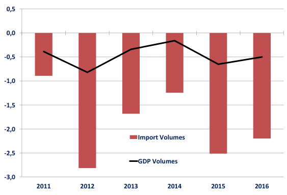
In 2016, global trade growth fell short of expectations for the sixth year in a row (Figure 1), fuelling a debate that resembles that on the Great Trade Collapse of 2008 and 2009 (Baldwin 2009). As with that debate, the recent dismal performance of trade has been attributed to structural factors such as the resurgence of protectionism, retrenchment of global value chains, the weakness of trade credit, and possible geographic or sectoral composition effects (Borin and Mancini 2015, Hoekman 2016, IRC Trade Task Force 2016).

Figure 1 Forecast errors on the growth of world import and world GDP volumes

Source: Author calculations based on IMF data.
Notes: Percentage-point difference between the growth rate at year t as reported in the IMF World Economic Outlook (WEO) published in October at year t+1 (actual data) and the growth rate at year t as predicted in the IMF WEO published in October at year t-1 (forecast). For the year 2016, actual data come from the IMF WEO Update published in January 2017.

The IMF estimated world trade volumes to grow at an annual average of 5.1% in 2011-2016, but their actual growth rate has been just 3.2% per year. Only one third of this systematic forecast error reflects lower-than-expected real GDP growth. The other two-thirds is explained by the fall of the income elasticity of trade (‘income elasticity’), defined as the ratio between real import growth and real GDP growth. Income elasticity has decreased from its historical average of 1.3, as implicit in the IMF’s forecasts to less than 1.0.¹

In a new paper we show, however, that due to two standard properties of real trade flows – their high volatility and their pro-cyclicality – income elasticity is itself a cyclical variable (Borin et al. 2017). In particular, when real GDP growth is positive but lower than its long-run trend, then the income elasticity of trade is also smaller than its long-run trend. This is important because it suggests that part of the decline in the income elasticity may be due to poor business conditions. Once this is factored in, we find that cyclical forces explain most of the current weakness of trade. In addition, we show that, by using real-time data on business conditions, the accuracy of forecasts on trade growth – like those produced by the IMF – can be significantly improved.

Trade Weakness: The Cycle and the Trend

Our research highlights the importance of income elasticity and shows, empirically and theoretically, that it is affected by business conditions.[2] At the empirical level we find a robust positive correlation with business cycle proxies (our preferred one being real investment growth).³ At a theoretical level, cyclicality arises because trade volumes are procyclical and more volatile than real GDP. The higher volatility of trade is, in turn, due to its different composition relative to GDP: trade is intensive in capital goods and manufactured goods, which are more volatile than consumption goods and services. Consumption goods and services, in turn, make up most of GDP and are less responsive to business conditions (think, for example, of public spending in education or health). Our paper demonstrates that this composition effect is responsible for the cyclical movements of the elasticity and drives it above (below) its trend following stronger (weaker) GDP growth.

Intuitively, suppose that GDP and import volumes grow at identical positive rates, say 3%, and focus only on positive growth rates. As real import growth is more volatile than, and positively correlated with, real GDP growth, when real GDP growth is above its average (say 4%), the important growth is even higher (say 5%). When real GDP growth is below its average (say 2%), real import growth is even lower (say 1%). Therefore, income elasticity will be greater than 1 when real GDP growth is high, and smaller than 1 when real GDP growth is low (5/4 and 1/2, respectively, in this simple numerical example). Thus, the income elasticity is procyclical.⁴

From the theoretical model, we can identify two main components of the income elasticity:

• A long-run component, related to the dynamics of trade barriers; and
• A short-run component, related to business cycle conditions.

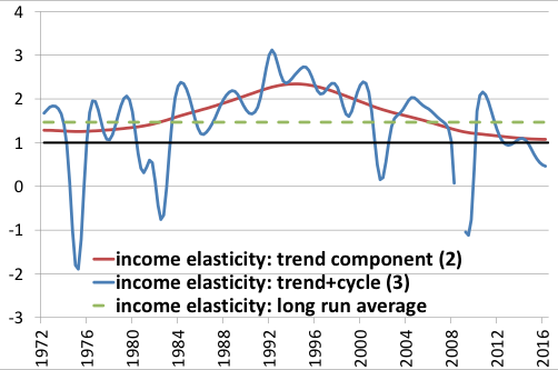
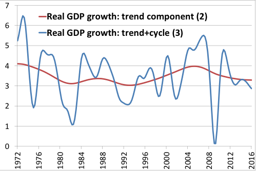
Figure 2a shows that for the global economy both these components are currently declining, helping depress trade relative to GDP. The long-run component highlights that trade volumes increased faster than real GDP in the 1980s and early 1990s, favoured by the secular decline in tariffs and in information and transportation costs. Since the late 1990s, however, this component has started to decrease, as the effect of falling trade barriers began to fade away. The cyclical component, which has always fluctuated around the long-run component, is currently driving the income elasticity below 1 (the equilibrium level of the elasticity, if there are no changes in trade barriers), because world real GDP growth is weak (Figure 2b).

Figure 2 Decomposition of the income elasticity of world trade and of world real GDP growth

a) Income elasticity

b) Real GDP growth

Source: Author calculations based on IMF data.
Notes: Quarterly data, 4-quarter moving averages. The picture excludes three consecutive outliers, from 2008-Q4 to 2009-Q2. (2) Trend component of the income elasticity from HP filtered series. (3) “Trend+cycle” component of the income elasticity from HP filtered series.

It is also worth noting that before the crisis (2002 to 2008) and in its immediate aftermath (Q3 2009 to Q2 2011), the cyclical component pushed the elasticity well above its long-run trend, hiding the fact that structural factors were already lowering the elasticity. This ‘optical illusion’ may also explain why the recent weakness of trade has been such a surprise.

These findings allow us to assess the role of cyclical and structural factors. Figure 2a shows that, with respect to its historical average of 1.5 (during our sample period), income elasticity has been reduced to 0.7 in 2015 with a similar contribution of structural and cyclical factors. But given that lower-than-expected GDP growth has also contributed a third of the forecast error, this back-of-the-envelope calculation suggests that cyclical forces have caused about two thirds of the forecast error – a result in line with the IMF’s estimate (Aslam et al. 2017).

Figure 2a also shows the trend component of the income elasticity stabilising at 1, which should remain similar until new impetus comes from further trade liberalisations or technological progress in transportation. Nevertheless, the exceptional weakness of global trade observed since 2011, which has gradually driven the income elasticity below 1, is also the result of poor business conditions. Therefore, one should expect that, as real GDP growth returns to trend, global trade growth recovers more strongly, with the income elasticity first returning to 1 and then exceeding this value once real GDP moves above its own trend growth.

Forecasting Trade

Our analysis speculates about the medium- to long-term future of global trade. What about the short term? Can we exploit data on business conditions to improve trade forecasts? We examined these questions by focusing on the forecasts of world import growth produced by the IMF – the most commonly used in the business community and among policymakers.

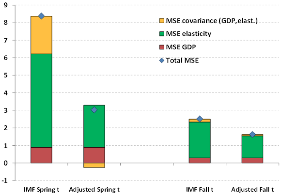
First, we decompose the mean squared forecast error (MSFE) on world trade growth into three terms which measure the forecast error on GDP growth (MSFE GDP), the forecast error on the income elasticity (MSFE elasticity), and the interaction between these two errors (MSFE covariance). We do this for the forecasts published by the IMF in the spring and fall of each calendar year t.⁵ The results show that the MSFE on the income elasticity is the largest component at all forecast horizons. In addition, as the forecast horizon shortens, the IMF improves its forecasts of world real GDP growth significantly, but not its forecast of the income elasticity.

The importance of the elasticity forecast error and of its correlation with GDP forecast error suggests that IMF forecasts can be improved by considering business cycle conditions. To prove our claim, we perform an out-of-sample forecasting exercise. We first estimate the role of the cycle using past data, considering different real-time proxies for business conditions. We then use regression results to ‘correct’ the IMF predictions. Figure 3 compares the MSFE using the IMF predictions and our cyclically-adjusted predictions. Using the cyclically adjusted predictions, forecast error declines substantially. For the forecasts produced in the spring, the total MSFE is cut by 70%, with half of the reduction coming from the improved prediction of the elasticity and half from the lower covariance between the elasticity forecast error and the GDP forecast error. For the autumn forecasts, the total MSFE is cut by 40%, with the reduction coming almost entirely from the improvement in predicting the elasticity. The effectiveness of our correction for the business cycle is reflected in the fact that the covariance between elasticity and GDP forecast errors becomes essentially nil.

Figure 3 Comparison between forecast errors, IMF and cyclically adjusted predictions

Source: Author calculations based on IMF data.
Notes: Total mean squared forecast error on world import growth in year t and its components, for the predictions made by the IMF in the spring and autumn of year t and for the corresponding cyclically adjusted predictions.

No More Illusions?

Our analysis identifies the structural and cyclical components that drive the behaviour of the income elasticity of trade. Since the mid-1990s, the structural component has been gradually declining towards its equilibrium level of 1. This result suggests that the income elasticity will probably not get close to the values of 2 or more recorded in the early 1990s unless international trade receives new impetus from international integration or technological advances in transportation. It could fall below 1 if, instead, trade liberalisation reversed.

At the same time, however, the analysis stresses the role of cyclical factors in the slowdown of trade in the current phase. One should then expect that, as real GDP growth returned to trend, global trade growth would recover more strongly, with the income elasticity first approaching, and then exceeding, 1 when real GDP growth moves above trend.