How Far Goods Travel: Global Transport and Supply Chains from 1965-2020

Yves here. Hopefully readers will chew over some of the interesting data about supply chains and different measures of activity, such as shipment distances, weight and value.

Perhaps I am reading too much into this post, but I am bothered by what I see as the tactic assumption that high levels of international trade are a new normal that will persist, with the evidence being that even the 2008 financial crisis had less of an impact that widely assumed. The wee problem here is, as Nassim Nicholas Taleb would be wont to point out, is tail risks. The world has a high level of international trade before World War I, and that broke down in the Great War. We see that the supposedly unsophisticated Houthis are already interfering with seaborne trade quite effectively, albeit only on certain routes. However, as today’s Links show, the alternate traffic path, around the horn of Africa, is currently stalled by severe weather. And while we are at it, what about global warming as another wild card, both via increasing the risk of seaborne trade and flooding or storm damage of key ports?

Reader reactions as always encouraged.

By Sharat Ganapati, Assistant Professor of International Economics Georgetown University and Woan Foong Wong, Assistant Professor University Of Oregon. Originally published at VoxEU

Disruptions from conflicts, climate change, and the pandemic have raised the question of whether today’s supply chains and transportation networks more resilient or vulnerable. This column examines the evolution of transport use and costs over the last 55 years, and its implications for international trade and supply chains. Goods are now transported by more countries over longer distances, driven by natural resources and raw materials versus downstream manufactured goods. While longer distance networks involving multiple countries may seem more susceptible to disruptions, the findings suggest a more nuanced take: countries are more cohesively interconnected because of the interaction between efficient transport, trade, and supply chains.

The creation of global supply chains relies on affordable and reliable transportation networks. Disruptions from conflicts, climate change, and pandemics have sparked a key question: are today’s supply chains and transportation networks more resilient or vulnerable? With supply chains constantly evolving and facing new challenges, it is essential to understand how global trade and the recovery capabilities of industries and countries may be affected by unforeseen disruptions (Alfaro and Chor 2023, Baldwin and Freeman 2020, 2022, Pandalai-Nayar et al. 2022).

In a recent paper (Ganapati and Wong 2023), we show the evolution of transport use and costs over the last 55 years, and its implications for international trade and supply chains. Goods are transported by more countries over longer distances, driven by natural resources and raw materials versus downstream manufactured goods. While longer distance networks involving multiple countries may seem more susceptible to disruptions, our findings suggest a more nuanced take: countries are more cohesively interconnected because of the interaction between efficient transport, trade, and supply chains. We emphasise the importance of considering (1) the global gains from increased transport reliability and use of trade, and (2) how local disruptions to production can have wide-reaching consequences through these interactions.

Global transportation increased dramatically from 1965 to 2020; more goods are being shipped and shipped further. Transportation services consist of two components: the amount of goods that are transported, and how far these goods are transported. Transport use can be measured either by weight (tonne-kilometres) per the transportation literature, ¹ or by value (dollar-kilometres) per the trade literature. While weight-based measures are reflective of low value-per-weight ratio goods like grain or petroleum products, value-based measures instead emphasise high value-per-weight goods like machinery and electronics. Multiplying both by distance measures transportation use, which is missing in traditional trade measures that just sum exports and imports.

Figure 1 shows international transportation trends from 1965 to 2020 and how they compare to conventional trade statistics. ² Transport use in weight (black solid line) has more than doubled over the past 50 years, reflecting the transport of raw materials. This transport increase is even larger when using value measures (grey dashed line), tripling from 1965 to 2007 before declining. Comparing these trends to conventional trade measures, which do not account for distance, allows us to highlight distance’s role over this period. Are more goods being shipped to countries that are further apart?

Figure 1 Transport use relative to total world output, 1965-2020

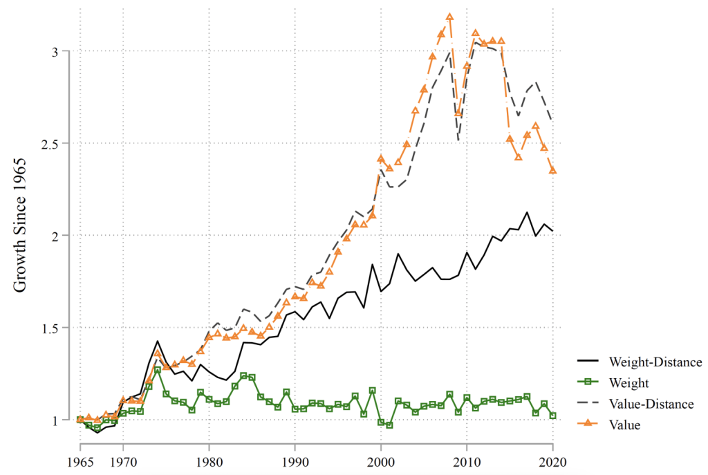
Notes: Trends are relative to the sum of the gross domestic product of all countries. All series are normalized with respect to its 1965 value and can be read as growth since 1965. The black line measures the distance shipped of goods, weighted by metric tons. The dashed grey line measures the distance shipped of goods, weighted by dollars. The green squares are the total weight shipped relative to World GDP. The orange triangles are the value shipped relative to World GDP. All monetary values are converted to year 2000 USD.
Source: Ganapati and Wong (2024)

We emphasise three themes.  First, when trade is measured by value, transport usage growth as a share of global output in dollar-distance (grey dashed line) echoes trade value growth (orange triangles), more than tripling from 1965 to 2007 before decreasing after the Great Recession (Eaton et al. 2016, Baldwin and Evenett 2009). In value, goods are being shipped more to both nearby and distant locations.

Second, when trade is measured by weight, transport usage growth as a share of global output in weight-distance (black solid line) is quite different from trade weight growth (green squares). The aggregate tonnage shipped stayed relatively constant from 1965 to 2020. Relative to the global economy, nations are not trading more goods by weight. However, when nations do trade these goods, they are transported over increasingly further distances.

Third, the growth in our distance-based trade statistics paralleled each other until 1990. After 1990, the value measure of trade accelerated through 2007 and then collapsed after the Great Recession. Meanwhile, the weight measure of transport rises steadily, largely unaffected by the recession.

This highlights differences in transportation economics and international trade. While conventional valued-based measures of trade collapsed following the Great Recession (Figure 1), transportation usage by weight and distance barely changed. Transport costs are typically treated as exogenous in international trade – approximated by distance and the ‘iceberg’ functional form, where the value of shipped goods decreases (‘melts’) with distance. ³ In contrast, in transportation economics the pricing structure is often at the per-unit level – for example, cost per tonne or container. These transport prices and costs are equilibrium outcomes, jointly determined with trade and transport use. Both the assumptions of exogeneity and iceberg functional form, while providing tractability in most trade models, have nontrivial trade and welfare implications (Hummels et al. 2009, Heiland et al. 2019, Brancaccio et al. 2020, Ganapati et al. 2021).

Second, we show that global transport costs have declined over the last half century (consistent with Hummels 2007 and Harrigan 2010). Using total expenditures in the transportation sector, we estimate upper and lower bound transport costs by weight and value. The cost to transport one ton of goods for one kilometre decreased by about 35% over this period (grey dotted lines in Figure 2). This trend exhibits significant volatility from 1975-1985, reflecting the price of oil due to OPEC supply restrictions. The cost of transporting a dollar’s worth of goods for one kilometre has decreased by over 50% (red solid lines in Figure 2), falling faster than when trade is measured by weights.

Figure 2 Transport costs, 1965-2014

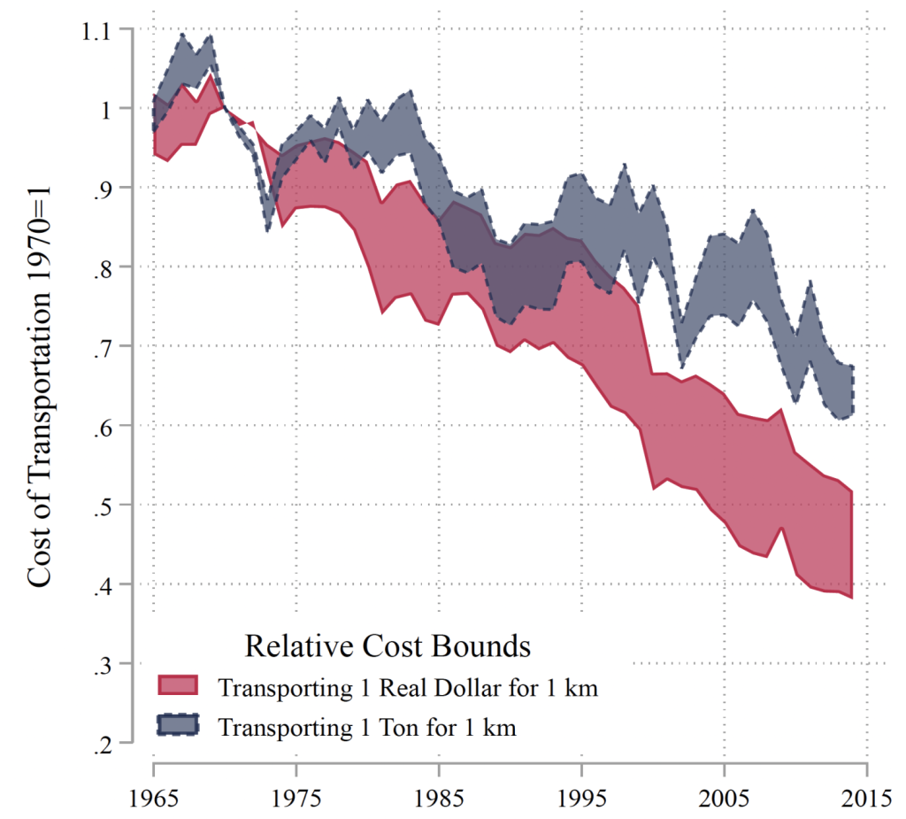
Notes: Figure 2 is calculated using the sum of all global transportation costs for a given year, divided by trade use for that year – either tonnes of trade or value of trade, multiplied by distance. For transportation costs, we use data on transportation and storage expenditures.  The upper bound estimate is based on the scenario where all aggregate transportation spending was on international trade while the lower bound estimate reflects spending on both international and domestic trade. Values are normalised to 1 in 1970. Consistent sample of 24 countries representing 90% of world GDP.
Source: Ganapati and Wong (2024)

The utilisation of transport services is an equilibrium response to its cost. Decreases in transport costs alter the terms of the classic proximity-concentration trade-off: firms can either expand production across borders to maximise proximity to foreign customers, or concentrate a production step in one location in order to benefit from economies of scale and export to many foreign destinations. Firms have broadly not maximised proximity to end users. Instead, they have expanded and even fragmented their production supply chains, altering the geographic location of economic activity (Antràs and Chor 2022, Redding 2022) or relying on lower transportation costs to expand exports. ⁴

What contributed to the large transport use increases since 1965? We emphasise three factors: (1) increasing participation of China; (2) increasing long distance trade; and (3) shifts in the composition of traded goods – upstream natural resources versus downstream manufactured goods.

Developing countries account for about 40% of world exports (UNCTAD 2022), driven by China. By recomputing our statistics without China, we show that all post-1990 transportation growth by weight reflects China’s emergence (Figure 3a). ⁵ But China plays a more moderate role in value-based measure of trade (Figure 3b). However, these high-value and low-weight goods may face changes in the proximity-concentration trade-off. As it becomes cheaper for raw materials to be imported, production locations reflect the location of final demand.

Figure 3 The role of emerging economies, focusing on China, 1965-2020

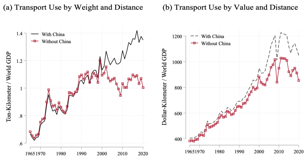
Notes: The real transport use measured in ton-distance, indicated by the black line in Figure 3a, is reproduced from Figure 1 in Ganapati and Wong (2024) for comparison. The real transport use measured in ton-distance excluding China, indicated by the red line with squares in Figure 3a, is calculated by recomputing Equation(2) in Appendix A to exclude both incoming and outgoing trade in weight with China in the numerator, as well as excluding Chinese GDP from world GDP in the denominator. The real transport use measured in dollar-distance, indicated by the black line in Figure 3b, is reproduced from Figure 1 in Ganapati and Wong (2024) for comparison. The real transport use measured in dollar-distance excluding China, indicated by the red line with squares in Figure 3a.
Source: Ganapati and Wong (2024)

Most of the weight-based transport use growth is due to increasing trade between countries that are further apart. Figure 4 breaks down our transport usage metrics from Figure 1 into three sub-components: the short distance bin for country pairs in the same region (within 5,000km); the medium distance bin (5,000-10,000km), which includes Asian-European trade; and the long distance bin, which includes Asia-North America trade.  While all bins contribute similar amounts by weight initially, transport use by countries that are further apart increased by more after the 1980s (Figure 4a).  Overall, longer-distance countries more than doubled their transport use. ⁶ Transport use by value instead shows large growth for all distances (Figure 4b). Overall, while heavier and lower value goods are being traded between countries that are further apart, lighter and higher value goods are being traded between locations that are both nearby and far apart.

Figure 4 The role of longer distance trade, 1965-2020

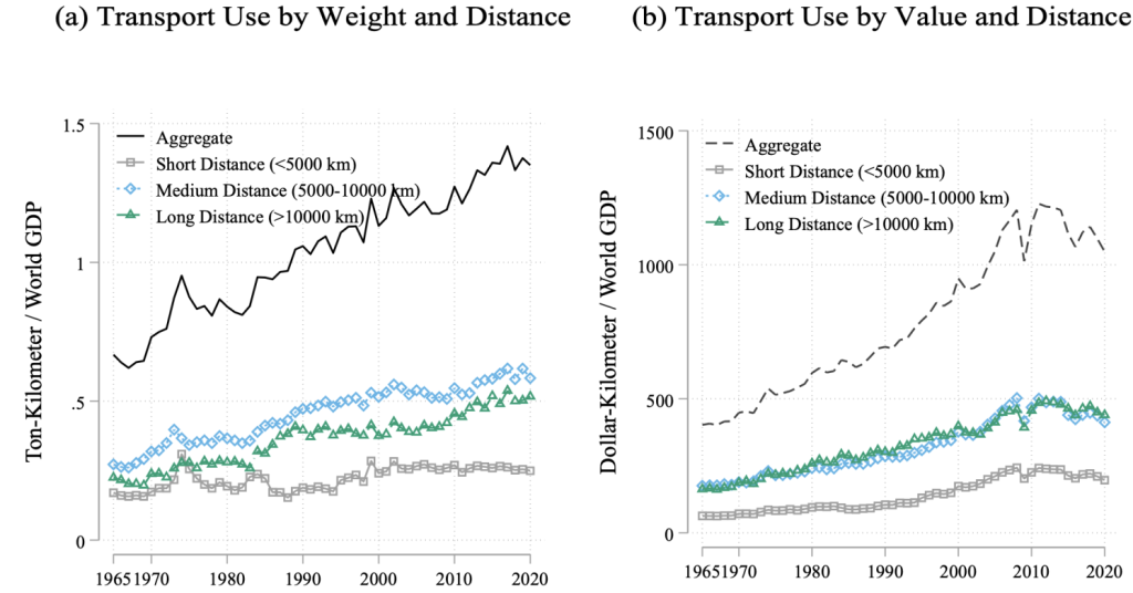
Notes: The real transport use measured in ton-distance, indicated by the black line in Figure 4a, is reproduced from Figure 1 in Ganapati and Wong (2024) for comparison. The remaining 3 lines in Figure 4a are calculated by breaking down the real transport use measure in weight into three sub-components that total the aggregate figures: transportation usage of shorter distance trade under 5,000 kilometres (grey line with squares), medium distance trade from 5,000 to 10,000 kilometres (blue line with diamonds), and very long distance trade over 10,000 kilometres (green line with triangles). The real transport use measured in dollar- distance, indicated by the black line in Figure 4b, is reproduced from Figure 1 in Ganapati and Wong (2024) for comparison. The remaining 3 lines in Figure 4b are calculated by breaking down the real transport use measure in value into three sub-components that total the aggregate figures.
Source: Ganapati and Wong (2024)

Lastly, we highlight the role of raw materials – that is, agricultural and natural resource products – relative to manufactured goods in Figure 5. From 1965-2000, both raw materials and manufactured goods equally contributed to transport use by weight (Figure 5a). Since 2000, however, manufactured goods no longer contribute to the growth in tonne-kilometres. Instead, all growth is due to raw materials.  These commodities are used as inputs into all production processes, are difficult to find substitutes for, and can be supplied by only a few countries (consistent with Fally and Sayre 2018). As the world economy grows, these indispensable raw materials are shipped farther distances (Berthelon and Freund 2008).  Even though raw materials are crucial required inputs, they constitute a much smaller share of total trade values (Figure 5b).

Figure 5 The role of natural resources vs manufactured goods, 1965-2020

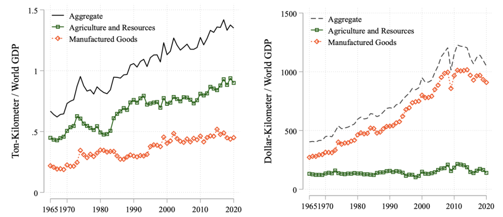
Notes: The real transport use measured in ton-distance, indicated by the solid black line in Figure 5a, is reproduced from Figure 1 in Ganapati and Wong (2024) for comparison. The remaining two lines in Figure 5a are calculated by breaking down the real transport use measure in weight into two sub-components that total the aggregate figure: agricultural and natural resource products (green line with squares), and manufactured products (orange line with diamonds). The real transport use measured in dollar-distance, indicated by the dashed black line in Figure 5b, is reproduced from Figure 1 in Ganapati and Wong (2024) for comparison. The remaining two lines in Figure 5b are calculated by breaking down the real transport use measure in value into two sub-components that total the aggregate figure: agricultural and natural resource products, and manufactured products.
Source: Ganapati and Wong (2024)

Over the past half century, goods have been transported over longer distances to more countries. While longer international networks spanning multiple countries might appear prone to disruptions (Attinasi et al 2024, Bai et al 2024), our data indicate a more nuanced perspective: when faced with the recent supply disruptions and congestion of the pandemic, firms and countries do not need to decrease their transport use. Instead, unexpected events teach lessons about unforeseen risks; for example, it is not only important for a firm to have multiple suppliers, but also to know that those suppliers can use multiple trade routes. Consolidating the entire supply chain at home is both costly and as risky, albeit in a different way, as a single-sourced foreign location. Researchers and policymakers should be able to study both sides of the coin: on one side, there are significant global gains from increased transport reliability and trade; on the other side, local disruptions can have far and wide-reaching consequences through the interactions of trading networks.

See original post for references